MNIST Tutorial#

Welcome to NNX! This tutorial will guide you through building and training a simple convolutional neural network (CNN) on the MNIST dataset using the NNX API. NNX is a Python neural network library built upon JAX and currently offered as an experimental module within Flax.

1. Install NNX#

Since NNX is under active development, we recommend using the latest version from the Flax GitHub repository:

!pip install git+https://github.com/google/flax.git

2. Load the MNIST Dataset#

We’ll use TensorFlow Datasets (TFDS) for loading and preparing the MNIST dataset:

import tensorflow_datasets as tfds  # TFDS for MNIST
import tensorflow as tf             # TensorFlow operations

tf.random.set_seed(0) # set random seed for reproducibility

num_epochs = 10
batch_size = 32

train_ds: tf.data.Dataset = tfds.load('mnist', split='train')
test_ds: tf.data.Dataset = tfds.load('mnist', split='test')

train_ds = train_ds.map(lambda sample: {
  'image': tf.cast(sample['image'],tf.float32) / 255,
  'label': sample['label']}) # normalize train set
test_ds = test_ds.map(lambda sample: {
  'image': tf.cast(sample['image'], tf.float32) / 255,
  'label': sample['label']}) # normalize test set

train_ds = train_ds.repeat(num_epochs).shuffle(1024) # create shuffled dataset by allocating a buffer size of 1024 to randomly draw elements from
train_ds = train_ds.batch(batch_size, drop_remainder=True).prefetch(1) # group into batches of batch_size and skip incomplete batch, prefetch the next sample to improve latency
test_ds = test_ds.shuffle(1024) # create shuffled dataset by allocating a buffer size of 1024 to randomly draw elements from
test_ds = test_ds.batch(batch_size, drop_remainder=True).prefetch(1) # group into batches of batch_size and skip incomplete batch, prefetch the next sample to improve latency

3. Define the Network with NNX#

Create a convolutional neural network with NNX by subclassing nnx.Module.

from flax.experimental import nnx  # NNX API

class CNN(nnx.Module):
  """A simple CNN model."""

  def __init__(self, *, rngs: nnx.Rngs):
    self.conv1 = nnx.Conv(in_features=1, out_features=32, kernel_size=(3, 3), rngs=rngs)
    self.conv2 = nnx.Conv(in_features=32, out_features=64, kernel_size=(3, 3), rngs=rngs)
    self.linear1 = nnx.Linear(in_features=3136, out_features=256, rngs=rngs)
    self.linear2 = nnx.Linear(in_features=256, out_features=10, rngs=rngs)

  def __call__(self, x):
    x = self.conv1(x)
    x = nnx.relu(x)
    x = nnx.avg_pool(x, window_shape=(2, 2), strides=(2, 2))
    x = self.conv2(x)
    x = nnx.relu(x)
    x = nnx.avg_pool(x, window_shape=(2, 2), strides=(2, 2))
    x = x.reshape((x.shape[0], -1))  # flatten
    x = self.linear1(x)
    x = nnx.relu(x)
    x = self.linear2(x)
    return x
  
model = CNN(rngs=nnx.Rngs(0))

print(f'model = {model}'[:500] + '\n...\n')  # print a part of the model
print(f'{model.conv1.kernel.shape = }') # inspect the shape of the kernel of the first convolutional layer

model = CNN(
  conv1=Conv(
    in_features=1,
    out_features=32,
    kernel_size=(3, 3),
    strides=1,
    padding=SAME,
    input_dilation=1,
    kernel_dilation=1,
    feature_group_count=1,
    use_bias=True,
    mask_fn=None,
    dtype=None,
    param_dtype=<class 'jax.numpy.float32'>,
    precision=None,
    kernel_init=<function variance_scaling.<locals>.init at 0x29b1149d0>,
    bias_init=<function zeros at 0x28547f0d0>,
    conv_general_dilated=<function conv_general_dilated at 0x2837
...

model.conv1.kernel.shape = (3, 3, 1, 32)

Run model#

Let’s put our model to the test! We’ll perform a forward pass with arbitrary data and print the results.

import jax
import jax.numpy as jnp  # JAX NumPy

y = model(jnp.ones((1, 28, 28, 1)))
y

Array([[ 0.4839074 ,  0.03281   , -0.17949843, -0.03062986, -0.27809557,
        -0.3449784 , -0.01757436, -0.8598586 ,  0.44058406, -0.36605638]],      dtype=float32)

4. Define Metrics#

To track our model’s performance, we’ll use the clu library. If you haven’t already, install it with:

!pip install -q clu

[notice] A new release of pip is available: 23.3.1 -> 24.0
[notice] To update, run: pip install --upgrade pip

Let’s create a compound metric using clu.metrics.Collection. This will include both an Accuracy metric for tracking how well our model classifies images, and an Average metric to monitor the average loss over each training epoch.

from clu import metrics
from flax import struct   # Flax pytree dataclasses

@struct.dataclass
class Metrics(metrics.Collection):
  accuracy: metrics.Accuracy
  loss: metrics.Average.from_output('loss')

5. Create the `TrainState`#

In Flax, a common practice is to use a dataclass to encapsulate the training state, including the step number, parameters, and optimizer state. The flax.training.train_state.TrainState class is ideal for basic use cases, simplifying the process by allowing you to pass a single argument to functions like train_step.

from flax.training import train_state  # Useful dataclass to keep train state
import optax  

params, static = model.split(nnx.Param)

class TrainState(train_state.TrainState):
  static: nnx.GraphDef[CNN]
  metrics: Metrics

learning_rate = 0.005
momentum = 0.9

tx = optax.adamw(learning_rate, momentum)
state = TrainState.create(
  apply_fn=None, params=params, tx=tx,
  static=static, metrics=Metrics.empty()
)

Since TrainState is a JAX pytree, Module.split splits the model into State and GraphDef pytree objects (representing parameters and the graph definition). A custom TrainState type holds the static GraphDef and metrics. We use optax to create an optimizer (adamw) and initialize the TrainState.

6. Training step#

This function takes the state and a data batch and does the following:

Reconstructs the model with static.merge on the params.
Runs the neural network on the input image batch.
Calculates cross-entropy loss using optax.softmax_cross_entropy_with_integer_labels(). Integer labels eliminate the need for one-hot encoding.
Computes the loss function’s gradient with jax.grad.
Updates model parameters by applying the gradient pytree to the optimizer.

@jax.jit
def train_step(state: TrainState, batch):
  """Train for a single step."""
  def loss_fn(params):
    model = state.static.merge(params)
    logits = model(batch['image'])
    loss = optax.softmax_cross_entropy_with_integer_labels(
        logits=logits, labels=batch['label']).mean()
    return loss
  grad_fn = jax.grad(loss_fn)
  grads = grad_fn(state.params)
  state = state.apply_gradients(grads=grads)
  return state

The @jax.jit decorator traces the train_step function for just-in-time compilation with XLA, optimizing performance on hardware accelerators.

7. Metric Computation#

Create a separate function to calculate loss and accuracy metrics. Loss is determined using the optax.softmax_cross_entropy_with_integer_labels function, and accuracy is computed using clu.metrics.

@jax.jit
def compute_metrics(*, state: TrainState, batch):
  model = state.static.merge(state.params)
  logits = model(batch['image'])
  loss = optax.softmax_cross_entropy_with_integer_labels(
        logits=logits, labels=batch['label']).mean()
  metric_updates = state.metrics.single_from_model_output(
    logits=logits, labels=batch['label'], loss=loss)
  metrics = state.metrics.merge(metric_updates)
  state = state.replace(metrics=metrics)
  return state

9. Seed randomness#

For reproducible dataset shuffling (using tf.data.Dataset.shuffle), set the TF random seed.

tf.random.set_seed(0)

10. Train and Evaluate#

Dataset Preparation: create a “shuffled” dataset

Repeat the dataset for the desired number of training epochs.
Establish a 1024-sample buffer (holding the dataset’s initial 1024 samples). Randomly draw batches from this buffer.
As samples are drawn, replenish the buffer with subsequent dataset samples.

Training Loop: Iterate through epochs

Sample batches randomly from the dataset.
Execute an optimization step for each training batch.
Calculate mean training metrics across batches within the epoch.
With updated parameters, compute metrics on the test set.
Log train and test metrics for visualization.

After 10 training and testing epochs, your model should reach approximately 99% accuracy.

num_steps_per_epoch = train_ds.cardinality().numpy() // num_epochs

metrics_history = {
  'train_loss': [],
  'train_accuracy': [],
  'test_loss': [],
  'test_accuracy': []
}

for step,batch in enumerate(train_ds.as_numpy_iterator()):
  # Run optimization steps over training batches and compute batch metrics
  state = train_step(state, batch) # get updated train state (which contains the updated parameters)
  state = compute_metrics(state=state, batch=batch) # aggregate batch metrics

  if (step+1) % num_steps_per_epoch == 0: # one training epoch has passed
    for metric,value in state.metrics.compute().items(): # compute metrics
      metrics_history[f'train_{metric}'].append(value) # record metrics
    state = state.replace(metrics=state.metrics.empty()) # reset train_metrics for next training epoch

    # Compute metrics on the test set after each training epoch
    test_state = state
    for test_batch in test_ds.as_numpy_iterator():
      test_state = compute_metrics(state=test_state, batch=test_batch)

    for metric,value in test_state.metrics.compute().items():
      metrics_history[f'test_{metric}'].append(value)

    print(f"train epoch: {(step+1) // num_steps_per_epoch}, "
          f"loss: {metrics_history['train_loss'][-1]}, "
          f"accuracy: {metrics_history['train_accuracy'][-1] * 100}")
    print(f"test epoch: {(step+1) // num_steps_per_epoch}, "
          f"loss: {metrics_history['test_loss'][-1]}, "
          f"accuracy: {metrics_history['test_accuracy'][-1] * 100}")

train epoch: 1, loss: 0.06638548523187637, accuracy: 98.1433334350586
test epoch: 1, loss: 0.04838135838508606, accuracy: 98.47756958007812
train epoch: 2, loss: 0.023823682218790054, accuracy: 99.35333251953125
test epoch: 2, loss: 0.0462910532951355, accuracy: 98.72796630859375
train epoch: 3, loss: 0.01530431304126978, accuracy: 99.62999725341797
test epoch: 3, loss: 0.03833530843257904, accuracy: 98.828125
train epoch: 4, loss: 0.009797323495149612, accuracy: 99.74666595458984
test epoch: 4, loss: 0.047368891537189484, accuracy: 98.71794891357422
train epoch: 5, loss: 0.007574543822556734, accuracy: 99.83666229248047
test epoch: 5, loss: 0.0390843003988266, accuracy: 99.0184326171875
train epoch: 6, loss: 0.006016132887452841, accuracy: 99.86499786376953
test epoch: 6, loss: 0.04912222921848297, accuracy: 98.828125
train epoch: 7, loss: 0.003792814677581191, accuracy: 99.90833282470703
test epoch: 7, loss: 0.07655340433120728, accuracy: 98.58773803710938
train epoch: 8, loss: 0.003739297855645418, accuracy: 99.9000015258789
test epoch: 8, loss: 0.07705188542604446, accuracy: 98.57772827148438
train epoch: 9, loss: 0.0030404471326619387, accuracy: 99.92832946777344
test epoch: 9, loss: 0.09123016148805618, accuracy: 98.32732391357422
train epoch: 10, loss: 0.0029481027740985155, accuracy: 99.91999816894531
test epoch: 10, loss: 0.07410085946321487, accuracy: 98.89823913574219

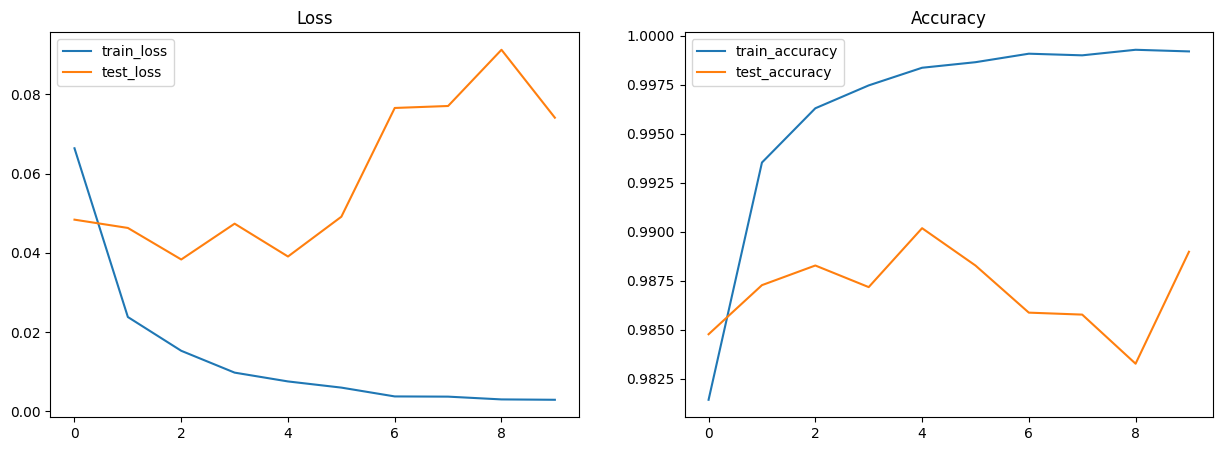
11. Visualize Metrics#

Use Matplotlib to create plots for loss and accuracy.

import matplotlib.pyplot as plt  # Visualization

# Plot loss and accuracy in subplots
fig, (ax1, ax2) = plt.subplots(1, 2, figsize=(15, 5))
ax1.set_title('Loss')
ax2.set_title('Accuracy')
for dataset in ('train','test'):
  ax1.plot(metrics_history[f'{dataset}_loss'], label=f'{dataset}_loss')
  ax2.plot(metrics_history[f'{dataset}_accuracy'], label=f'{dataset}_accuracy')
ax1.legend()
ax2.legend()
plt.show()
plt.clf()

../../_images/4db69fc053e583dd581e22d55bf9a25d988bb41f262a1fb5eb63c1c0e87055af.png

<Figure size 640x480 with 0 Axes>

12. Perform inference on test set#

Define a jitted inference function, pred_step, to generate predictions on the test set using the learned model parameters. This will enable you to visualize test images alongside their predicted labels for a qualitative assessment of model performance.

@jax.jit
def pred_step(state: TrainState, batch):
  model = state.static.merge(state.params)
  logits = model(test_batch['image'])
  return logits.argmax(axis=1)

test_batch = test_ds.as_numpy_iterator().next()
pred = pred_step(state, test_batch)

fig, axs = plt.subplots(5, 5, figsize=(12, 12))
for i, ax in enumerate(axs.flatten()):
    ax.imshow(test_batch['image'][i, ..., 0], cmap='gray')
    ax.set_title(f"label={pred[i]}")
    ax.axis('off')

../../_images/2a8f6e73a020a557d8be6e0ff4092473d3e7e6da95cc6eff48a3cf08eaf0a207.png

Congratulations! You made it to the end of the annotated MNIST example.

MNIST Tutorial

Contents